Zillow is one of the largest marketplaces for real estate information in the U.S. and a leading example of impactful machine learning (ML). Zillow Research uses ML models that analyze hundreds of data points on each property to estimate home values and predict market changes. In this chapter, we cover how to use Apache Spark ML Random Forest Regression to predict the median sales prices for homes in a region. Note that currently only XGBoost is GPU-Accelerated in Spark ML, which we will cover in the next chapter.
Predicting Housing Prices Using Apache Spark Machine Learning
Classification and Regression
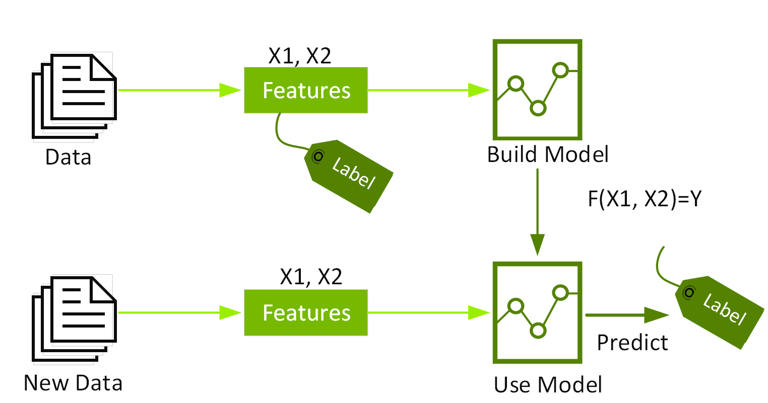
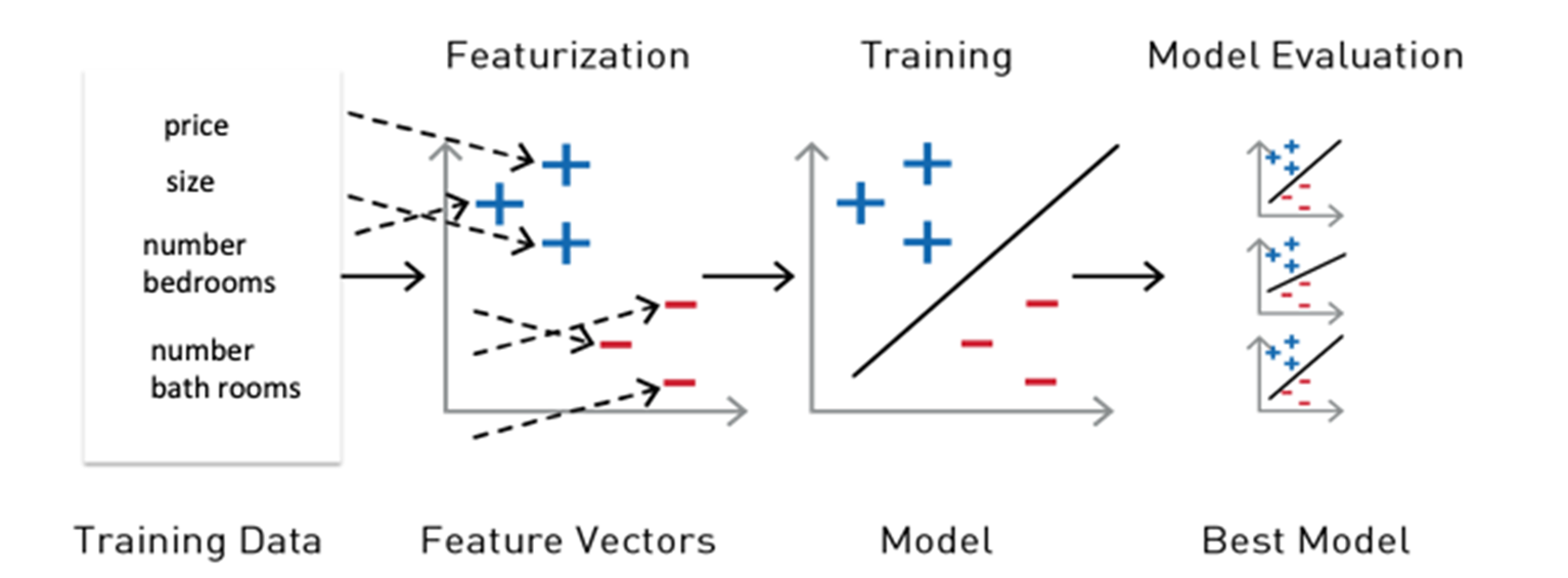
Classification and regression are two categories of supervised machine learning algorithms. Supervised ML, also called predictive analytics, uses algorithms to find patterns in labeled data and then uses a model that recognizes those patterns to predict the labels on new data. Classification and regression algorithms take a dataset with labels (also called the target outcome) and features (also called properties) and learn how to label new data based on those data features.
Classification identifies which category an item belongs to, such as whether a credit card transaction is legitimate. Regression predicts a continuous numeric value like a house price, for example.
Regression
Regression estimates the relationship between a target outcome dependent variable (the label) and one or more independent variables (the features). Regression can be used to analyze the strength of the relationship between the label and the feature variables, determine how much the label changes with an adjustment in one or more feature variables, and predict trends between the label and feature variables.
Let's go through a linear regression example of housing prices, given historical house prices and features of houses (square feet, number of bedrooms, location, etc.):
- What are we trying to predict?
This is the label: the house price - What are the data properties that you can use to predict?
These are the features: to build a regression model, you extract the features of interest that have the strongest relationship with the label and contribute the most to the prediction.
In the following example, we’ll use the size of the house.
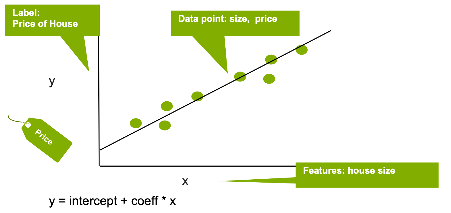
Linear regression models the relationship between the Y "Label" and the X "Feature", in this case the relationship between the house price and size, with the equation: Y = intercept + (coefficient * X) + error. The coefficient measures the impact of the feature on the label, in this case the impact of the house size on the price.
Multiple linear regression models the relationship between two or more "Features" and a "Label." For example, if we wanted to model the relationship between the price and the house size, the number of bedrooms, and the number of bathrooms, the multiple linear regression function would look like this:
Yi = β0 + β1X1 + β2X2 + · · · + βp Xp + Ɛ
Price = intercept + (coefficient1 size) + (coefficient2 bedrooms) + (coefficient3 * bathrooms) + error.
The coefficients measure the impact on the price of each of the features.
Decision Trees
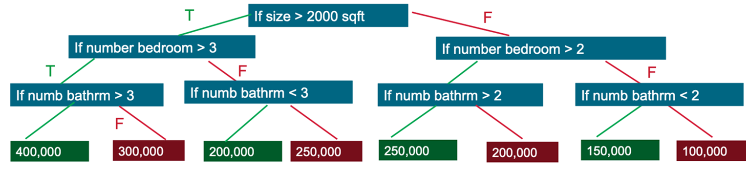
Decision trees create a model that predicts the label by evaluating a set of rules that follow an if-then-else pattern. The if-then-else feature questions are the nodes, and the answers “true” or “false” are the branches in the tree to the child nodes.
A decision tree model estimates the minimum number of true/false questions needed to assess the probability of making a correct decision. Decision trees can be used for classification to predict a category, or probability of a category, or regression to predict a continuous numeric value. Following is an example of a simplified decision tree to predict housing prices:
- Q1: If the size of the house > 2000sqft
- T:Q2: If the number of bedrooms > 3
- T:Q3: If the number of bathrooms is > 3
- T: Price=$400,000
- F: Price=$200,000
- T:Q3: If the number of bathrooms is > 3
- T:Q2: If the number of bedrooms > 3
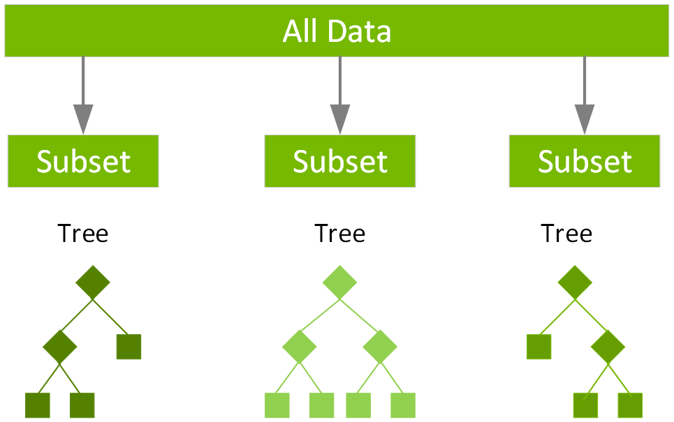
Random Forests
Ensemble learning algorithms combine multiple machine learning algorithms to obtain a better model. Random forest is a popular ensemble learning method for classification and regression. The algorithm builds a model consisting of multiple decision trees, based on different subsets of data at the training stage. Predictions are made by combining the output from all the trees, which reduces the variance and improves the predictive accuracy. For random forest classification, the label is predicted to be the class predicted by the majority of trees. For random forest regression, the label is the mean regression prediction of the individual trees.
Spark provides the following algorithms for regression:
- Linear regression
- Generalized linear regression
- Decision tree regression
- Random forest regression
- Gradient-boosted tree regression
- XGBoost regression
- Survival regression
- Isotonic regression
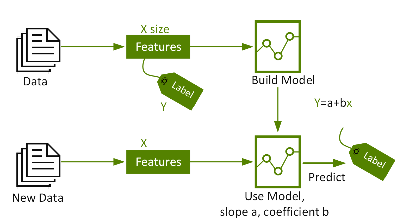
Machine Learning Workflows
Machine learning is an iterative process which involves:
- Extracting, Transforming, Loading (ETL) and analyzing historical data in order to extract the significant features and label.
- Training, testing, and evaluating the results of ML algorithms to build a model.
- Using the model in production with new data to make predictions.
- Model monitoring and model updating with new data.
Using Spark ML Pipelines
For the features and label to be used by an ML algorithm, they must be put into a feature vector, which is a vector of numbers representing the value for each feature. Feature vectors are used to train, test, and evaluate the results of an ML algorithm to build the best model.
Reference Learning Spark
Spark ML provides a uniform set of high-level APIs, built on top of DataFrames for building ML pipelines or workflows. Having ML pipelines built on top of DataFrames provides the scalability of partitioned data processing with the ease of SQL for data manipulation.
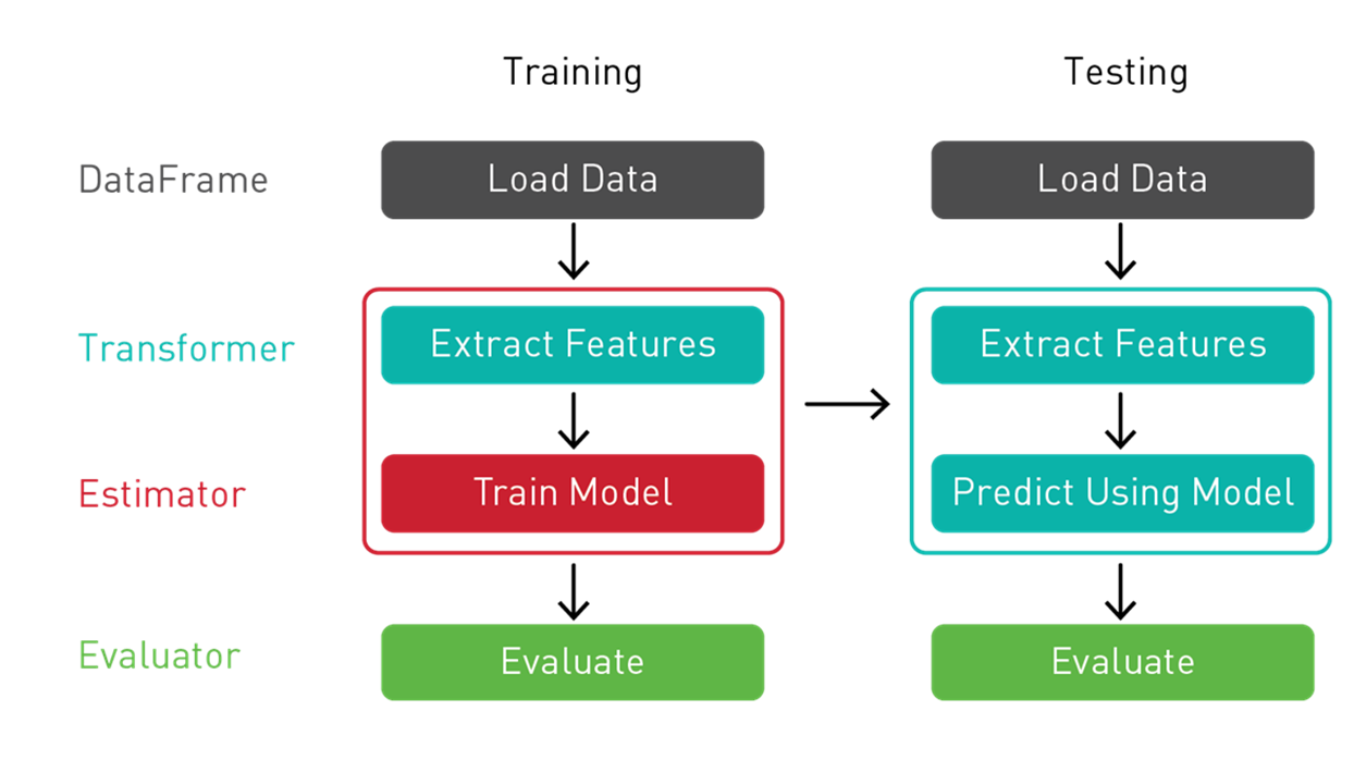
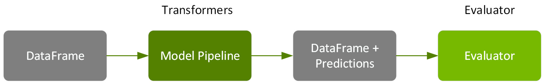
We use a Spark ML Pipeline to pass the data through transformers and extract the features, an estimator to produce the model, and an evaluator to measure the accuracy of the model.
- Transformer: A Transformer is an algorithm that transforms one DataFrame into another DataFrame. We’ll use a Transformer to create a DataFrame with a features vector column.
- Estimator: An Estimator is an algorithm that can be fit on a DataFrame to produce a transformer. We’ll use an estimator to train a model, and return a model Transformer, which can add a predictions column to a DataFrame with a features vector column.
- Pipeline: A pipeline chains multiple Transformers and Estimators together to specify an ML workflow.
- Evaluator: An Evaluator measures the accuracy of a trained Model on label and prediction DataFrame columns.
Example Use Case Dataset
In this example, we’ll be using the California housing prices dataset from the StatLib repository. This dataset contains 20,640 records based on data from the 1990 California census, with each record representing a geographic block. The following list provides a description for the attributes of the data set.
- Median House Value: Median house value (in thousands of dollars) for households within a block.
- Longitude: East/west measurement, a higher value is further west.
- Latitude: North/south measurement, a higher value is further north.
- Housing Median Age: Median age of a house within a block, lower is newer.
- Total Rooms: Total number of rooms within a block.
- Total Bedrooms: Total number of bedrooms within a block.
- Population: Total number of people residing within a block.
- Households: Total number of households in a block.
- Median Income: Median income for households within a block of houses (measured in tens of thousands of dollars).
To build a model, you extract the features that most contribute to the prediction. In order to make some of the features more relevant for predicting the median house value, instead of using totals we’ll calculate and use these ratios: rooms per house=total rooms/households, people per house=population/households, and bedrooms per rooms=total bedrooms/total rooms.
In this scenario, we use random forest regression on the following label and features:
- Label → median house value
- Features → {"median age", "median income", "rooms per house", "population per house", "bedrooms per room", "longitude", "latitude" }
Load the Data from a File into a DataFrame
The first step is to load our data into a DataFrame. In the following code, we specify the data source and schema to load into a dataset.
import org.apache.spark._
import org.apache.spark.ml._
import org.apache.spark.ml.feature._
import org.apache.spark.ml.regression._
import org.apache.spark.ml.evaluation._
import org.apache.spark.ml.tuning._
import org.apache.spark.sql._
import org.apache.spark.sql.functions._
import org.apache.spark.sql.types._
import org.apache.spark.ml.Pipeline
val schema = StructType(Array(
StructField("longitude", FloatType,true),
StructField("latitude", FloatType, true),
StructField("medage", FloatType, true),
StructField("totalrooms", FloatType, true),
StructField("totalbdrms", FloatType, true),
StructField("population", FloatType, true),
StructField("houshlds", FloatType, true),
StructField("medincome", FloatType, true),
StructField("medhvalue", FloatType, true)
))
var file ="/path/cal_housing.csv"
var df = spark.read.format("csv").option("inferSchema", "false").schema(schema).load(file)
df.show
result:
+---------+--------+------+----------+----------+----------+--------+---------+---------+
|longitude|latitude|medage|totalrooms|totalbdrms|population|houshlds|medincome|medhvalue|
+---------+--------+------+----------+----------+----------+--------+---------+---------+
| -122.23| 37.88| 41.0| 880.0| 129.0| 322.0| 126.0| 8.3252| 452600.0|
| -122.22| 37.86| 21.0| 7099.0| 1106.0| 2401.0| 1138.0| 8.3014| 358500.0|
| -122.24| 37.85| 52.0| 1467.0| 190.0| 496.0| 177.0| 7.2574| 352100.0|
+---------+--------+------+----------+----------+----------+--------+---------+---------+
In the following code example, we use the DataFrame withColumn() transformation, to add columns for the ratio features: rooms per house=total rooms/households, people per house=population/households, and bedrooms per rooms=total bedrooms/total rooms. We then cache the DataFrame and create a temporary view for better performance and ease of using SQL.
// create ratios for features
df = df.withColumn("roomsPhouse", col("totalrooms")/col("houshlds"))
df = df.withColumn("popPhouse", col("population")/col("houshlds"))
df = df.withColumn("bedrmsPRoom", col("totalbdrms")/col("totalrooms"))
df=df.drop("totalrooms","houshlds", "population" , "totalbdrms")
df.cache
df.createOrReplaceTempView("house")
spark.catalog.cacheTable("house")
Summary Statistics
Spark DataFrames include some built-in functions for statistical processing. The describe() function performs summary statistics calculations on numeric columns and returns them as a DataFrame. The following code shows some statistics for the label and some features.
df.describe("medincome","medhvalue","roomsPhouse","popPhouse").show
result:
+-------+------------------+------------------+------------------+------------------+
|summary| medincome| medhvalue| roomsPhouse| popPhouse|
+-------+------------------+------------------+------------------+------------------+
| count| 20640| 20640| 20640| 20640|
| mean|3.8706710030346416|206855.81690891474| 5.428999742190365| 3.070655159436382|
| stddev|1.8998217183639696|115395.61587441359|2.4741731394243205| 10.38604956221361|
| min| 0.4999| 14999.0|0.8461538461538461|0.6923076923076923|
| max| 15.0001| 500001.0| 141.9090909090909|1243.3333333333333|
+-------+------------------+------------------+------------------+------------------+
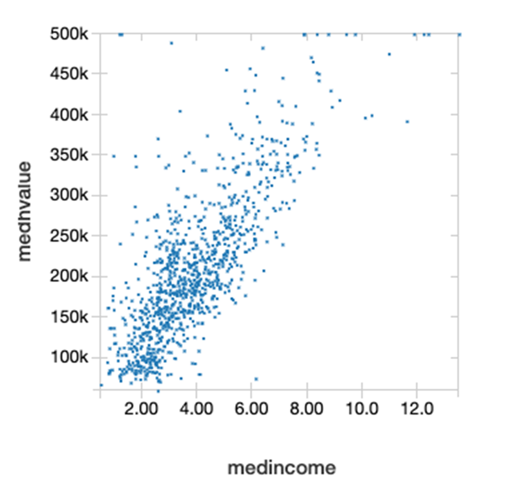
The DataFrame Corr() function calculates the Pearson correlation coefficient of two columns of a DataFrame. This measures the statistical relationship between two variables based on the method of covariance. Correlation coefficient values range from 1 to -1, where 1 indicates a perfect positive relationship, -1 indicates a perfect negative relationship, and a 0 indicates no relationship. Below we see that the median income and the median house value have a positive correlation relationship.
df.select(corr("medhvalue","medincome")).show()
+--------------------------+
|corr(medhvalue, medincome)|
+--------------------------+
| 0.688075207464692|
+--------------------------+
The following scatterplot of the median house value on the Y axis and median income on the X axis shows that they are linearly related to each other.
The following code uses the DataFrame randomSplit method to randomly split the Dataset into two, with 80% for training and 20% for testing.
val Array(trainingData, testData) = df.randomSplit(Array(0.8, 0.2), 1234)
Feature Extraction and Pipelining
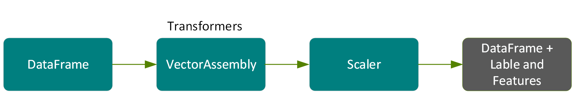
The following code creates a VectorAssembler (a transformer), which will be used in a pipeline to combine a given list of columns into a single feature vector column.
val featureCols = Array("medage", "medincome", "roomsPhouse", "popPhouse", "bedrmsPRoom", "longitude", "latitude")
//put features into a feature vector column
val assembler = new
VectorAssembler().setInputCols(featureCols).setOutputCol("rawfeatures")
The following code creates a StandardScaler (a transformer), which will be used in a pipeline to standardize features by scaling to unit variance using DataFrame column summary statistics.
val scaler = new
StandardScaler().setInputCol("rawfeatures").setOutputCol("features").setWithStd(true.setWithMean(true)
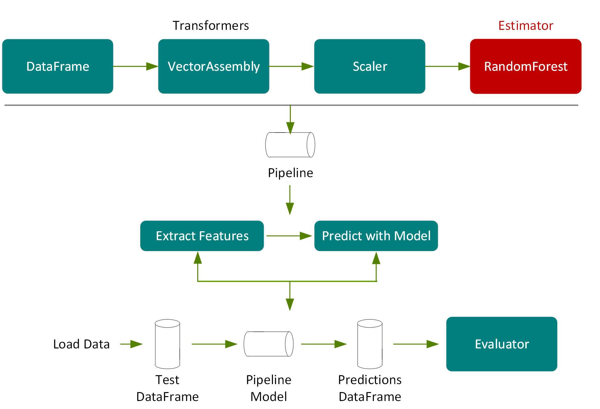
The result of running these transformers in a pipeline will be to add a scaled features column to the dataset as shown in the following figure.
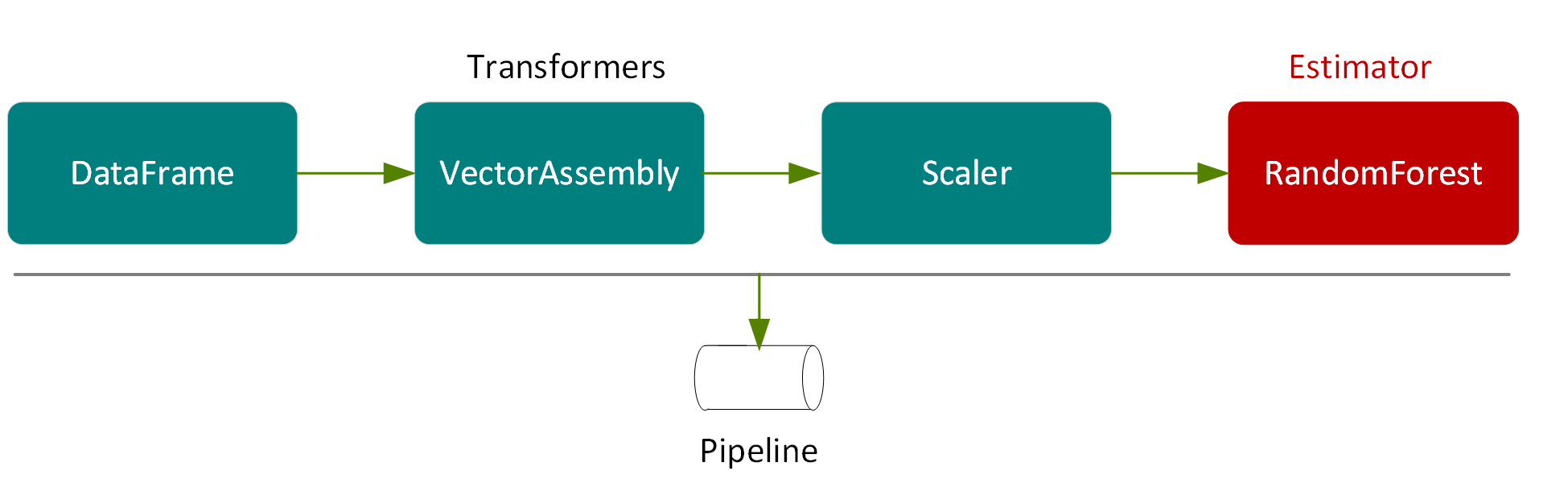
The final element in our pipeline is a RandomForestRegressor (an estimator), which trains on the vector of features and label, and then return a RandomForestRegressorModel (a transformer) .
val rf = new
RandomForestRegressor().setLabelCol("medhvalue").setFeaturesCol("features")
In the following example, we put the VectorAssembler, Scaler and RandomForestRegressor in a Pipeline. A pipeline chains multiple transformers and estimators together to specify an ML workflow for training and using a model.
val steps = Array(assembler, scaler, rf)
val pipeline = new Pipeline().setStages(steps)
Train the Model
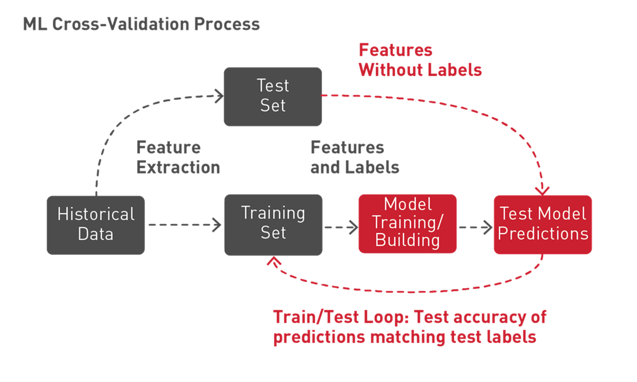
Spark ML supports a technique called k-fold cross-validation to try out different combinations of parameters in order to determine which parameter values of the ML algorithm produce the best model. With k-fold cross-validation, the data is randomly split into k partitions. Each partition is used once as the test dataset, while the rest are used for training. Models are then generated using the training sets and evaluated with the testing sets, resulting in k model accuracy measurements. The model parameters leading to the highest accuracy measurements produce the best model.
Spark ML supports k-fold cross-validation with a transformation/estimation pipeline which tries out different combinations of parameters, using a process called grid search, where you set up the parameters to test in a cross-validation workflow.
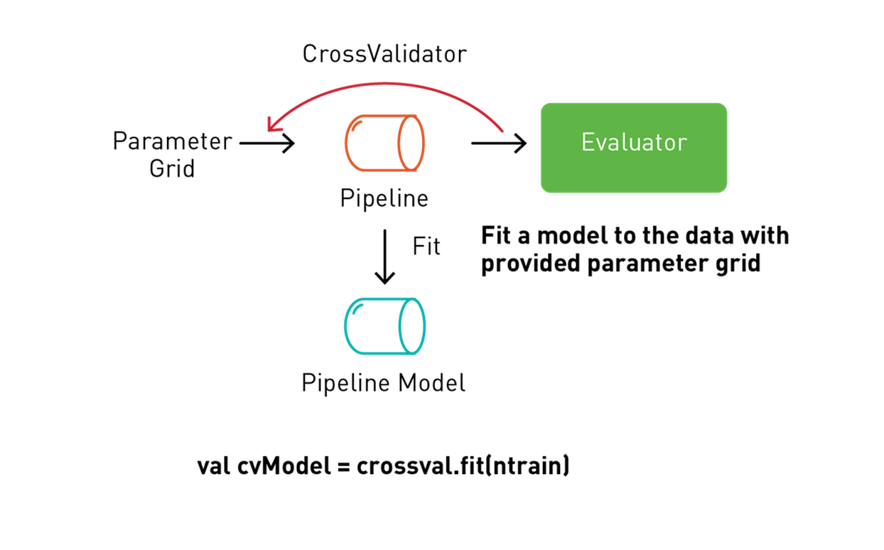
The following code uses a ParamGridBuilder to construct the parameter grid for the model training. We define a RegressionEvaluator, which will evaluate the model by comparing the test medhvalue column with the test prediction column. We use a CrossValidator for model selection. The CrossValidator uses the pipeline, the parameter grid, and the evaluator to fit the training dataset and return the best model. The CrossValidator uses the ParamGridBuilder to iterate through the maxDepth, maxBins, and numbTrees parameters of the RandomForestRegressor estimator and to evaluate the models, repeating three times per parameter value for reliable results.
val paramGrid = new ParamGridBuilder()
.addGrid(rf.maxBins, Array(100, 200))
.addGrid(rf.maxDepth, Array(2, 7, 10))
.addGrid(rf.numTrees, Array(5, 20))
.build()
val evaluator = new RegressionEvaluator()
.setLabelCol("medhvalue")
.setPredictionCol("prediction")
.setMetricName("rmse")
val crossvalidator = new CrossValidator()
.setEstimator(pipeline)
.setEvaluator(evaluator)
.setEstimatorParamMaps(paramGrid)
.setNumFolds(3)
// fit the training data set and return a model
val pipelineModel = crossvalidator.fit(trainingData)
Next, we can get the best model in order to print out the feature importances. The results show that the median income, population per house, and the longitude are the most important features.
val featureImportances = pipelineModel
.bestModel.asInstanceOf[PipelineModel]
.stages(2)
.asInstanceOf[RandomForestRegressionModel]
.featureImportances
assembler.getInputCols
.zip(featureImportances.toArray)
.sortBy(-_._2)
.foreach { case (feat, imp) =>
println(s"feature: $feat, importance: $imp") }
result:
feature: medincome, importance: 0.4531355014139285
feature: popPhouse, importance: 0.12807843645878508
feature: longitude, importance: 0.10501162983981065
feature: latitude, importance: 0.1044621179898163
feature: bedrmsPRoom, importance: 0.09720295935509805
feature: roomsPhouse, importance: 0.058427239343697555
feature: medage, importance: 0.05368211559886386
In the following example we get the parameters for the best random forest model produced, using the cross-validation process, which returns: max depth of 2, max bins of 50 and 5 trees.
val bestEstimatorParamMap = pipelineModel
.getEstimatorParamMaps
.zip(pipelineModel.avgMetrics)
.maxBy(_._2)
._1
println(s"Best params:\n$bestEstimatorParamMap")
result:
rfr_maxBins: 50,
rfr_maxDepth: 2,
rfr_-numTrees: 5
Predictions and Model Evaluation
Next we use the test DataFrame, which was a 20% random split of the original DataFrame, and was not used for training, to measure the accuracy of the model.
In the following code we call transform on the pipeline model, which will pass the test DataFrame, according to the pipeline steps, through the feature extraction stage, estimate with the random forest model chosen by model tuning, and then return the predictions in a column of a new DataFrame.
val predictions = pipelineModel.transform(testData)
predictions.select("prediction", "medhvalue").show(5)
result:
+------------------+---------+
| prediction|medhvalue|
+------------------+---------+
|104349.59677450571| 94600.0|
| 77530.43231856065| 85800.0|
|111369.71756877871| 90100.0|
| 97351.87386020401| 82800.0|
+------------------+---------+
With the predictions and labels from the test data, we can now evaluate the model. To evaluate the linear regression model, you measure how close the predictions values are to the label values. The error in a prediction, shown by the green lines below, is the difference between the prediction (the regression line Y value) and the actual Y value, or label. (Error = prediction-label).
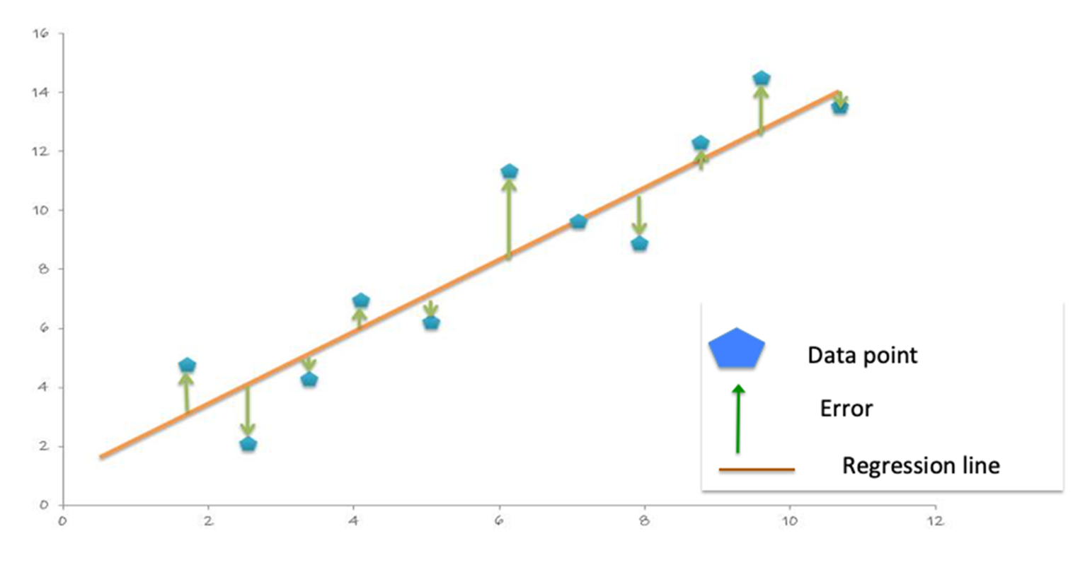
The Mean Absolute Error (MAE) is the mean of the absolute difference between the label and the model’s predictions. The absolute removes any negative signs.
MAE = sum(absolute(prediction-label)) / number of observations).
The Mean Square Error (MSE) is the sum of the squared errors divided by the number of observations. The squaring removes any negative signs and also gives more weight to larger differences. (MSE = sum(squared(prediction-label)) / number of observations).
The Root Mean Squared Error (RMSE) is the square root of the MSE. RMSE is the standard deviation of the prediction errors. The Error is a measure of how far from the regression line label data points are and RMSE is a measure of how spread out these errors are.
The following code example uses the DataFrame withColumn transformation, to add a column for the error in prediction: error=prediction-medhvalue. Then we display the summary statistics for the prediction, the median house value, and the error (in thousands of dollars).
predictions = predictions.withColumn("error",
col("prediction")-col("medhvalue"))
predictions.select("prediction", "medhvalue", "error").show
result:
+------------------+---------+-------------------+
| prediction|medhvalue| error|
+------------------+---------+-------------------+
| 104349.5967745057| 94600.0| 9749.596774505713|
| 77530.4323185606| 85800.0| -8269.567681439352|
| 101253.3225967887| 103600.0| -2346.677403211302|
+------------------+---------+-------------------+
predictions.describe("prediction", "medhvalue", "error").show
result:
+-------+-----------------+------------------+------------------+
|summary| prediction| medhvalue| error|
+-------+-----------------+------------------+------------------+
| count| 4161| 4161| 4161|
| mean|206307.4865123929|205547.72650805095| 759.7600043416329|
| stddev|97133.45817381598|114708.03790345002| 52725.56329678355|
| min|56471.09903814694| 26900.0|-339450.5381565819|
| max|499238.1371374392| 500001.0|293793.71945819416|
+-------+-----------------+------------------+------------------+
The following code example uses the Spark RegressionEvaluator to calculate the MAE on the predictions DataFrame, which returns 36636.35 (in thousands of dollars).
val maevaluator = new RegressionEvaluator()
.setLabelCol("medhvalue")
.setMetricName("mae")
val mae = maevaluator.evaluate(predictions)
result:
mae: Double = 36636.35
The following code example uses the Spark RegressionEvaluator to calculate the RMSE on the predictions DataFrame, which returns 52724.70.
val evaluator = new RegressionEvaluator()
.setLabelCol("medhvalue")
.setMetricName("rmse")
val rmse = evaluator.evaluate(predictions)
result:
rmse: Double = 52724.70
Save the Model
We can now save our fitted pipeline model to the distributed file store for later use in production. This saves both the feature extraction stage and the random forest model chosen by model tuning.
pipelineModel.write.overwrite().save(modeldir)
The result of saving the pipeline model is a JSON file for metadata and a Parquet for model data. We can reload the model with the load command; the original and reloaded models are the same:
val sameModel = CrossValidatorModel.load(“modeldir")
Summary
In this chapter, we discussed Regression, Decision Trees, and Random Forest algorithms. We covered the fundamentals of Spark ML pipelines and worked through a real world example to predict median house prices.