Introduction to Apache Spark Processing

IDC predicts that data generated in data centers, as well as from edge computing and IOT, will quintuple in the next seven years to 175 ZB. In tandem with the monumental growth of data, Apache Spark from Apache Software Foundation has become one of the most popular frameworks for distributed scale-out data processing, running on millions of servers—both on premises and in the cloud. This chapter provides an introduction to the Spark framework and explains how it executes applications.

Apache Spark is a fast and general purpose analytics engine for large-scale data processing, that runs on Hadoop, Apache Mesos, Kubernetes, standalone, or in the cloud. Spark offers high-level operators that make it easy to build parallel applications in Scala, Python, R, or SQL, using an interactive shell, notebooks, or packaged applications.

On top of the Spark core data processing engine, there exist libraries for SQL and DataFrames, machine learning, GraphX, graph computation, and stream processing. These libraries can be used together on massive datasets from a variety of data sources, such as HDFS, Alluxio, Apache Cassandra, Apache HBase, or Apache Hive.

How Spark Executes on a Cluster

A Spark application runs as parallel tasks inside of executor processes on cluster nodes, with execution coordinated between the SparkSession object in the driver program and the Resource or Cluster manager (either Standalone, Mesos, YARN, or Kubernetes) on the cluster.

Spark can also run on a single machine, called local mode. In local mode, the driver program and the tasks run in threads in the same Java Virtual Machine. Local mode is useful for prototyping, development, debugging and testing. However local mode is not meant for running production applications.

Creating a DataFrame from a File

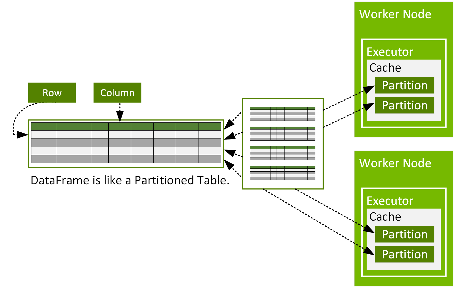
A Spark DataFrame is a distributed Dataset of org.apache.spark.sql.Row objects, that are partitioned across multiple nodes in a cluster and can be operated on in parallel. A DataFrame represents a table of data with rows and columns, similar to a DataFrame in R or Python, but with Spark optimizations. A DataFrame consists of partitions, each of which is a range of rows in cache on a data node.

DataFrames can be constructed from data sources, such as csv, parquet, JSON files, Hive tables, or external databases. A DataFrame can be operated on using relational transformations and Spark SQL queries.

The Spark shell or Spark notebooks provide a simple way to use Spark interactively. You can start the shell in local mode with the following command:

$ /[installation path]/bin/spark-shell --master local[2]

You can then enter the code from the rest of this chapter into the shell to see the results interactively. In the code examples, the outputs from the shell are prefaced with the result.

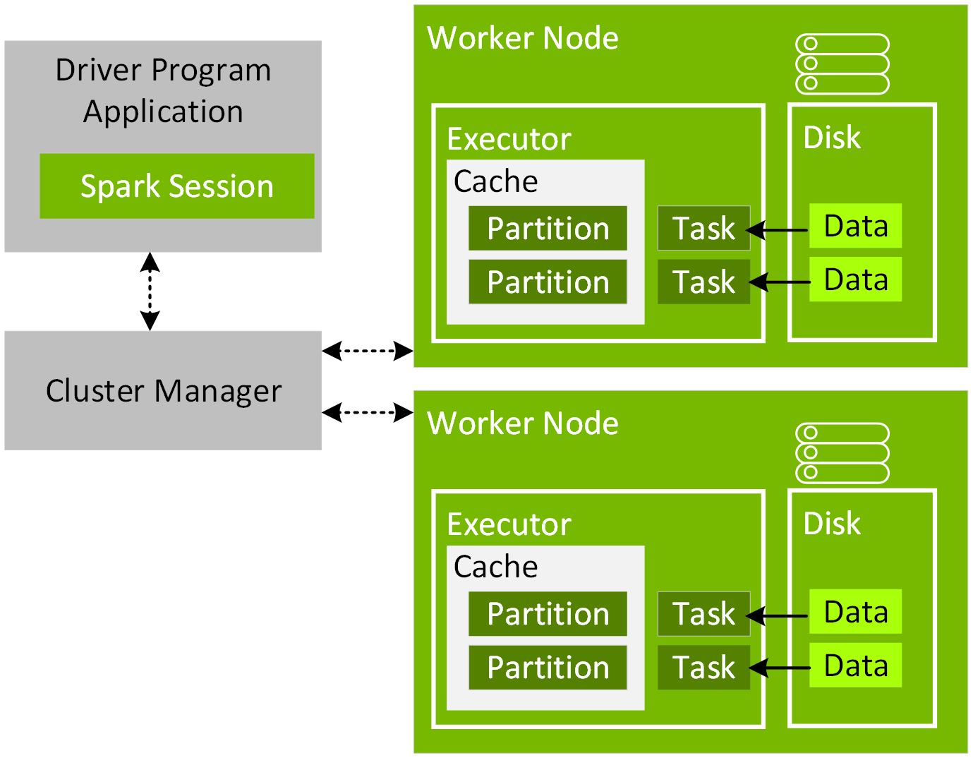
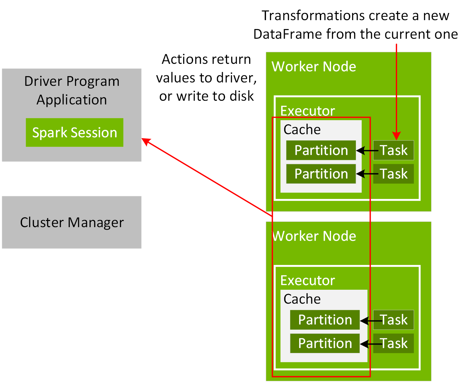
For execution coordination between your application driver and the Cluster manager, you create a SparkSession object in your program, as shown in the following code example:

val spark = SparkSession.builder.appName("Simple Application").master("local[2]").getOrCreate()

When a Spark application starts, it connects to the cluster manager via the master URL. The master URL can be set to the cluster manager or local[N] to run locally with N threads, when creating the SparkSession object or when submitting the Spark application. When using the spark-shell or notebook, the SparkSession object is already created and available as the variable spark. Once connected, the cluster manager allocates resources and launches executor processes, as configured for the nodes in your cluster. When a Spark application executes, the SparkSession sends tasks to the executors to run.

With the SparkSession read method, you can read data from a file into a DataFrame, specifying the file type, file path, and input options for the schema.

import org.apache.spark.sql.types._
import org.apache.spark.sql._
import org.apache.spark.sql.functions._

val schema =
  StructType(Array(
    StructField("vendor_id", DoubleType),
    StructField("passenger_count", DoubleType),
    StructField("trip_distance", DoubleType),
    StructField("pickup_longitude", DoubleType),
    StructField("pickup_latitude", DoubleType),
    StructField("rate_code", DoubleType),
    StructField("store_and_fwd", DoubleType),
    StructField("dropoff_longitude", DoubleType),
    StructField("dropoff_latitude", DoubleType),
    StructField("fare_amount", DoubleType),
    StructField("hour", DoubleType),
    StructField("year", IntegerType),
    StructField("month", IntegerType),
    StructField("day", DoubleType),
    StructField("day_of_week", DoubleType),
    StructField("is_weekend", DoubleType)
  ))

val file = "/data/taxi_small.csv"

val df = spark.read.option("inferSchema", "false")
.option("header", true).schema(schema).csv(file)

result:
df: org.apache.spark.sql.DataFrame = [vendor_id: double, passenger_count:
double ... 14 more fields]

The take method returns an array with objects from this DataFrame, which we see is of the org.apache.spark.sql.Row type.

df.take(1)
result:
Array[org.apache.spark.sql.Row] =
Array([4.52563162E8,5.0,2.72,-73.948132,40.829826999999995,-6.77418915E8,-1.0,-73.969648,40.797472000000006,11.5,10.0,2012,11,13.0,6.0,1.0])

DataFrame Transformations and Actions

DataFrames provide a domain-specific language API for structured data processing, known as transformations. Transformations create a new transformed DataFrame from the current DataFrame and are lazily evaluated. Transformations are executed when triggered by an action, which returns a result to the driver program or writes to disk. Once an action has run and the value is returned, the DataFrame is no longer in memory, unless it is cached. Spark can cache DataFrames using an in-memory columnar format by calling dataFrame.cache().

Here is a list of some commonly used DataFrame transformations.

select Selects a set of columns
join Join with another DataFrame, using the given join expression
groupBy Groups the DataFrame, using the specified columns

This groupBy transformation example groups the taxi DataFrame by hour of the day, then the count action totals the number of taxi trips for each hour. The show action prints out the resulting DataFrame rows in a tabular format.

df.groupBy("hour").count().show(4)

result:
+----+-----+
|hour|count|
+----+-----+
| 0.0| 12|
| 1.0| 49|
| 2.0| 658|
| 3.0| 742|
+----+-----+

Following is a list of some commonly used DataFrame actions.

show(n) Displays the first n rows in a tabular format
take(n) Returns the first n rows in the DataFrame in an array
count Returns the number of rows in the DataFrame

DataFrame Transformation Narrow and Wide Dependencies

There are two types of DataFrame transformations, those with narrow dependencies and those with wide dependencies. Transformations with narrow dependencies do not have to move data between partitions when creating a new DataFrame from an existing one. An example narrow transformation is filter() which is used to filter the rows from a DataFrame based on the given SQL expression. The following example filters for the hour value = 0.

Multiple narrow transformations can be performed on a DataFrame in memory, using a process called pipelining, making narrow transformations very efficient. Narrow transformations like filter and select are used in the example below to retrieve taxi fare_amounts for the 0 hour of the day.

// select and filter are narrow transformations
df.select($"hour", $"fare_amount").filter($"hour" === "0.0" ).show(2)

result:
+----+-----------+
|hour|fare_amount|
+----+-----------+
| 0.0| 10.5|
| 0.0| 12.5|
+----+-----------+

Transformations with wide dependencies have to move data between partitions, when creating a new DataFrame from an existing one, in a process called a shuffle. Shuffles send data across the network to other nodes and write to disk, causing network and disk I/O. Example wide transformations are groupBy, agg, sortBy, and orderBy. The wide transformation shows groups by the hour value.

Following is a wide transformation to group by the hour value and count the number of taxi trips by hour.

df.groupBy("hour").count().show(4)

result:
+----+-----+
|hour|count|
+----+-----+
| 0.0| 12|
| 1.0| 49|
| 2.0| 658|
| 3.0| 742|
+----+-----+

Please fill out the form below to keep reading this E-book

Section

Section

First Name

Last Name

Business Email Address

Organization / University Name

Location

Preferred Language

State/Province

enterpriseOptIns hidden field

Send me the latest enterprise news, announcements, and more from NVIDIA. I can unsubscribe at any time.

NVIDIA Privacy Policy

本人知悉且同意 NVIDIA 基于调研、活动组织的目的对本人的上述信息的收集和处理，并已经阅读并同意 <a href="https://www.nvidia.cn/about-nvidia/privacy-policy/?deeplink=visiting-our-website" target="_blank">NVIDIA 隐私政策</a>。

本人知悉且同意，因调研、活动组织的必须，以及相对应的 NVIDIA 内部管理和系统操作的需要，上述信息会被传输到位于美国的 NVIDIA Corporation 按照符合 <a href="https://www.nvidia.cn/about-nvidia/privacy-policy/?deeplink=visiting-our-website" target="_blank">NVIDIA 隐私政策</a>的方式进行存储，您可以通过发送邮件至 <a href="mailto:privacy@nvidia.com">privacy@nvidia.com</a> 进行联系以解决相关问题，实现可适用的数据保护法所规定的权利。