Predicting Taxi Fares Using GPU-Accelerated XGBoost

Big data is one of the 10 major areas used to improve cities. The analysis of location and behavior patterns within cities allows for optimization of traffic, better planning decisions, and smarter advertising. For example, the analysis of GPS car data enables cities to optimize traffic flows based on real-time traffic information. Telecom companies are using mobile phone location data to provide insights by identifying and predicting the location activity trends and patterns of a population in large metropolitan areas. And, the application of machine learning (ML) to geolocation data is proving instrumental in identifying patterns and trends for the telecom, travel, marketing, and manufacturing industries.

In this chapter, we’ll use public New York taxi trip data to examine regression analysis on taxi trip data as it pertains to predicting NYC taxi fares. We’ll start with an overview of the XGBoost algorithm and then explore the use case.

XGBoost

XGBoost, which stands for Extreme Gradient Boosting, is a scalable, distributed gradient-boosted decision tree (GBDT) machine learning library. XGBoost provides parallel tree boosting and is the leading ML library for regression, classification, and ranking problems. The RAPIDS team works closely with the Distributed Machine Learning Common (DMLC) XGBoost organization, and XGBoost now includes seamless, drop-in GPU acceleration, significantly speeding up model training and improving accuracy for better predictions.

Gradient Boosting Decision Trees (GBDTs) is a decision tree ensemble algorithm similar to Random Forest, the difference is in how the trees are built and combined. Random Forest uses a technique called bagging to build full decision trees in parallel from bootstrap samples of the data set. The final prediction is an average of all of the decision tree predictions. Gradient Boosting Decision Trees use a technique called boosting to iteratively train an ensemble of shallow decision trees, with each iteration using weights given to records in the previous sample, which did not predict correctly, to decrease the error of the succeeding tree. The final prediction is a weighted average of all of the decision tree predictions. Bagging minimizes the variance and overfitting, boosting minimizes the bias and underfitting.

XGBoost is a variation of GBDTs. With GBDTs, the decision trees are built sequentially. With XGBoost, trees are built in parallel, following a level-wise strategy, scanning across gradient values and using these partial sums to evaluate the quality of splits at every possible split in the training set.

GPU-Accelerated XGBoost

The GPU-accelerated XGBoost algorithm makes use of fast parallel prefix sum operations to scan through all possible splits, as well as parallel radix sorting to repartition data. It builds a decision tree for a given boosting iteration, one level at a time, processing the entire Dataset concurrently on the GPU.

GPU-accelerated Spark XGBoost offers the following key features:

Partitioning of ORC, CSV, and Parquet input files across multi GPUs
Essentially any number/size of supported input file formats can be divided up evenly among the different training nodes.
GPU-accelerated training
Improved XGBoost training time with a dynamic in-memory representation of the training data that optimally stores features based on the sparsity of a dataset rather than a fixed in-memory representation based on the largest number of features amongst different training instances. Decision trees are built using gradient pairs that can be reused to save memory, reducing copies to increase performance.
Efficient GPU memory utilization
XGBoost requires data to fit into memory which creates a restriction on data size using either a single GPU or distributed multi-GPU multi-node training. Now, with improved GPU memory utilization, users can train with five times the size of data as compared to the first version. This is one of the critical factors to improve total cost of training without impacting performance.

Example Use Case Dataset

The example dataset is a New York Taxi Dataset, which has already been cleaned up and transformed to add features, such as the haversine distance using this Spark ETL notebook.

In this scenario, we’ll build a model to predict the taxi fare amount, based on the following features:

Label 🡪 fare amount
Features 🡪 {passenger count, trip distance, pickup longitude, pickup latitude, rate code, dropoff longitude, dropoff latitude, hour, day of week, is weekend}

Load the Data from a File into a DataFrame

First, we import the packages needed for both GPU version and CPU versions of Spark xgboost:

import org.apache.spark.sql.functions._
import org.apache.spark.sql.types._
import org.apache.spark.sql._
import org.apache.spark.ml._
import org.apache.spark.ml.feature._
import org.apache.spark.ml.evaluation._
import org.apache.spark.sql.types._
import ml.dmlc.xgboost4j.scala.spark.{XGBoostRegressor, XGBoostRegressionModel}

For the GPU version of Spark xgboost you also need the following import:

import ml.dmlc.xgboost4j.scala.spark.rapids.{GpuDataReader, GpuDataset}

We specify the schema with a Spark StructType.

lazy val schema =
  StructType(Array(
    StructField("vendor_id", DoubleType),
    StructField("passenger_count", DoubleType),
    StructField("trip_distance", DoubleType),
    StructField("pickup_longitude", DoubleType),
    StructField("pickup_latitude", DoubleType),
    StructField("rate_code", DoubleType),
    StructField("store_and_fwd", DoubleType),
    StructField("dropoff_longitude", DoubleType),
    StructField("dropoff_latitude", DoubleType),
    StructField(labelName, DoubleType),
    StructField("hour", DoubleType),
    StructField("year", IntegerType),
    StructField("month", IntegerType),
    StructField("day", DoubleType),
    StructField("day_of_week", DoubleType),
    StructField("is_weekend", DoubleType)
  ))

In the following code we create a Spark session and set the training and evaluation data file paths. (Note: If you are using a notebook, then you do not have to create the SparkSession.)

val trainPath = "/FileStore/tables/taxi_tsmall.csv"
val evalPath = "/FileStore/tables/taxi_esmall.csv"
val spark = SparkSession.builder().appName("Taxi-GPU").getOrCreate

We load the data from a CSV file into a Spark DataFrame, specifying the datasource and schema to load into a DataFrame, as shown below.

val tdf = spark.read.option("inferSchema",
"false").option("header", true).schema(schema).csv(trainPath)
val edf = spark.read.option("inferSchema", "false").option("header",
true).schema(schema).csv(evalPath)

DataFrame show(5) displays the first 5 rows:

tdf.select("trip_distance", "rate_code","fare_amount").show(5)
result:
+------------------+-------------+-----------+
| trip_distance| rate_code|fare_amount|
+------------------+-------------+-----------+
| 2.72|-6.77418915E8| 11.5|
| 0.94|-6.77418915E8| 5.5|
| 3.63|-6.77418915E8| 13.0|
| 11.86|-6.77418915E8| 33.5|
| 3.03|-6.77418915E8| 11.0|
+------------------+-------------+-----------+

The function describe returns a DataFrame containing descriptive summary statistics, such as count, mean, standard deviation, and minimum and maximum value for each numerical column.

tdf.select("trip_distance", "rate_code","fare_amount").describe().show
+-------+------------------+--------------------+------------------+
|summary| trip_distance| rate_code| fare_amount|
+-------+------------------+--------------------+------------------+
| count| 7999| 7999| 7999|
| mean| 3.278923615451919|-6.569284350812602E8|12.348543567945994|
| stddev|3.6320775770793547|1.6677419425906155E8|10.221929466939088|
| min| 0.0| -6.77418915E8| 2.5|
| max|35.970000000000006| 1.957796822E9| 107.5|
+-------+------------------+--------------------+------------------+

The following scatter plot is used to explore the correlation between the fare amount and the trip distance.

%sql
select trip_distance, fare_amount
from taxi

Define Features Array

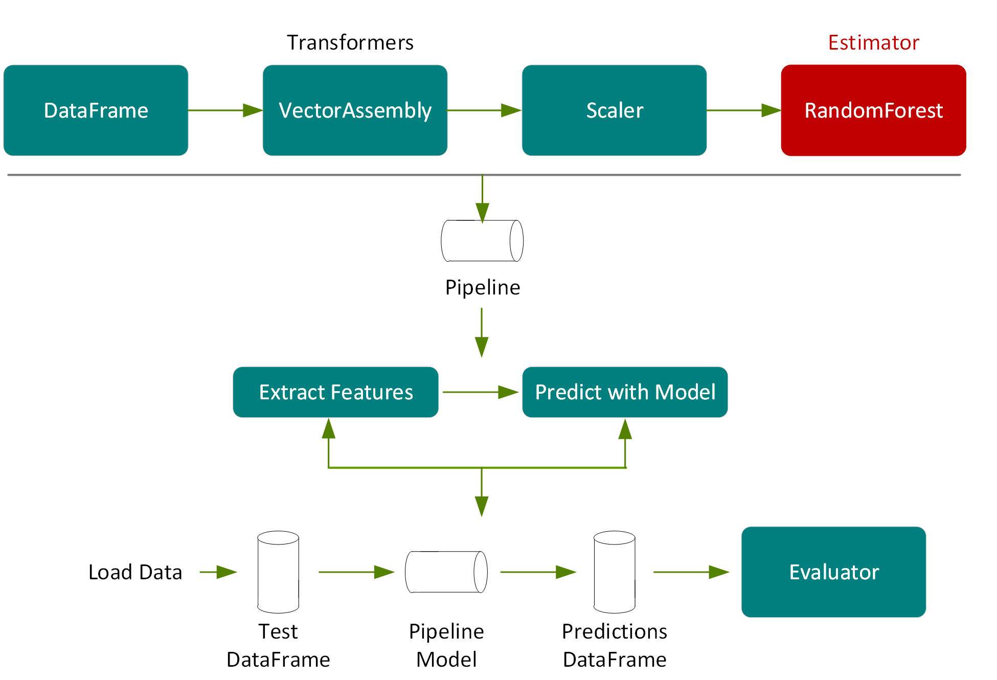
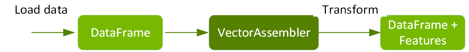
For the features to be used by an ML algorithm, they are transformed and put into feature vectors, which are vectors of numbers representing the value for each feature. Below, a VectorAssembler transformer is used to return a new DataFrame with a label and a vector features column.

// feature column names
val featureNames = Array("passenger_count","trip_distance", "pickup_longitude","pickup_latitude","rate_code","dropoff_longitude", "dropoff_latitude", "hour", "day_of_week","is_weekend")
// create transformer
object Vectorize {
  def apply(df: DataFrame, featureNames: Seq[String], labelName: String): DataFrame = {
    val toFloat = df.schema.map(f => col(f.name).cast(FloatType))
    new VectorAssembler()
      .setInputCols(featureNames.toArray)
      .setOutputCol("features")
      .transform(df.select(toFloat:_*))
      .select(col("features"), col(labelName))
  }
}
// transform method adds features column
var trainSet = Vectorize(tdf, featureNames, labelName)
var evalSet = Vectorize(edf, featureNames, labelName)
trainSet.take(1)
result:
res8: Array[org.apache.spark.sql.Row] =
Array([[5.0,2.7200000286102295,-73.94813537597656,40.82982635498047,-6.77418944E8,-73.96965026855469,40.79747009277344,10.0,6.0,1.0],11.5])

When using the XGBoost GPU version, the VectorAssembler is not needed.

For the CPU version the num_workers should be set to the number of CPU cores, the tree_method to “hist,” and the features column to the output features column in the Vector Assembler.

lazy val paramMap = Map(
  "learning_rate" -> 0.05,
  "max_depth" -> 8,
  "subsample" -> 0.8,
  "gamma" -> 1,
  "num_round" -> 500
)
// set up xgboost parameters
val xgbParamFinal = paramMap ++ Map("tree_method" -> "hist", "num_workers" -> 12)
// create the xgboostregressor estimator
val xgbRegressor = new XGBoostRegressor(xgbParamFinal)
      .setLabelCol(labelName)
      .setFeaturesCol("features")

For the GPU version the num_workers should be set to the number of machines with GPU in the Spark cluster, the tree_method to “gpu_hist,” and the features column to an array of strings containing the feature names.

val xgbParamFinal = paramMap ++ Map("tree_method" -> "gpu_hist",
"num_workers" -> 1)
// create the estimator
val xgbRegressor = new XGBoostRegressor(xgbParamFinal)
.setLabelCol(labelName)
.setFeaturesCols(featureNames)

The following code uses the XGBoostRegressor estimator fit method on the training dataset to train and return an XGBoostRegressor model. We also use a time method to return the time to train the model and we use this to compare the time training with CPU vs. GPU.

object Benchmark {
  def time[R](phase: String)(block: => R): (R, Float) = {
    val t0 = System.currentTimeMillis
    val result = block // call-by-name
    val t1 = System.currentTimeMillis
    println("Elapsed time [" + phase + "]: " +
    ((t1 - t0).toFloat / 1000) + "s")
    (result, (t1 - t0).toFloat / 1000)
  }
}
// use the estimator to fit (train) a model
val (model, _) = Benchmark.time("train") {
  xgbRegressor.fit(trainSet)
}

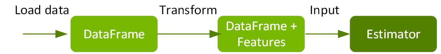
The performance of the model can be evaluated using the eval dataset which has not been used for training. We get predictions on the test data using the model transform method.

The model will estimate with the trained XGBoost model, and then return the fare amount predictions in a new predictions column of the returned DataFrame. Here again, we use the Benchmark time method in order to compare prediction times.

val (prediction, _) = Benchmark.time("transform") {
  val ret = model.transform(evalSet).cache()
  ret.foreachPartition(_ => ())
  ret
}
prediction.select( labelName, "prediction").show(10)
Result:
+-----------+------------------+
|fare_amount| prediction|
+-----------+------------------+
| 5.0| 4.749197959899902|
| 34.0|38.651187896728516|
| 10.0|11.101678848266602|
| 16.5| 17.23284912109375|
| 7.0| 8.149757385253906|
| 7.5|7.5153608322143555|
| 5.5| 7.248467922210693|
| 2.5|12.289423942565918|
| 9.5|10.893491744995117|
| 12.0| 12.06682014465332|
+-----------+------------------+

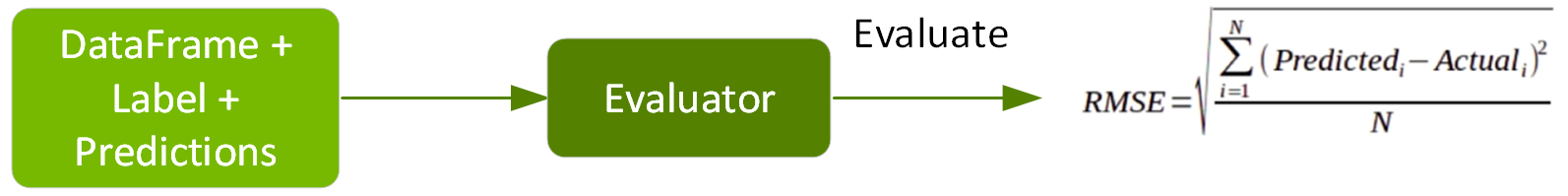
The RegressionEvaluator evaluate method calculates the root mean square error, which is the square root of the mean squared error, from the prediction and label columns.

val evaluator = new RegressionEvaluator().setLabelCol(labelName)
val (rmse, _) = Benchmark.time("evaluation") {
evaluator.evaluate(prediction)
}
println(s"RMSE == $rmse")
Result:
Elapsed time [evaluation]: 0.356s
RMSE == 2.6105287283128353

Save the Model

The model can be saved to disk, as shown below, in order to use later.

model.write.overwrite().save(savepath)

The result of saving the model is a JSON file for metadata and a Parquet file for model data. We can reload the model with the load command. The original and reloaded models are the same.

val sameModel = XGBoostRegressionModel.load(savepath)

Summary

In this chapter, we covered the basics of how XGBoost works and how to use XGBoost Regression with Spark to predict taxi fare amounts. You can now run this example on CPUs and GPUs with a larger dataset to compare time and accuracy of predictions.

Please fill out the form below to keep reading this E-book

Section

Section

First Name

Last Name

Business Email Address

Organization / University Name

Location

Preferred Language

State/Province

enterpriseOptIns hidden field

Send me the latest enterprise news, announcements, and more from NVIDIA. I can unsubscribe at any time.

NVIDIA Privacy Policy

本人知悉且同意 NVIDIA 基于调研、活动组织的目的对本人的上述信息的收集和处理，并已经阅读并同意 <a href="https://www.nvidia.cn/about-nvidia/privacy-policy/?deeplink=visiting-our-website" target="_blank">NVIDIA 隐私政策</a>。

本人知悉且同意，因调研、活动组织的必须，以及相对应的 NVIDIA 内部管理和系统操作的需要，上述信息会被传输到位于美国的 NVIDIA Corporation 按照符合 <a href="https://www.nvidia.cn/about-nvidia/privacy-policy/?deeplink=visiting-our-website" target="_blank">NVIDIA 隐私政策</a>的方式进行存储，您可以通过发送邮件至 <a href="mailto:privacy@nvidia.com">privacy@nvidia.com</a> 进行联系以解决相关问题，实现可适用的数据保护法所规定的权利。