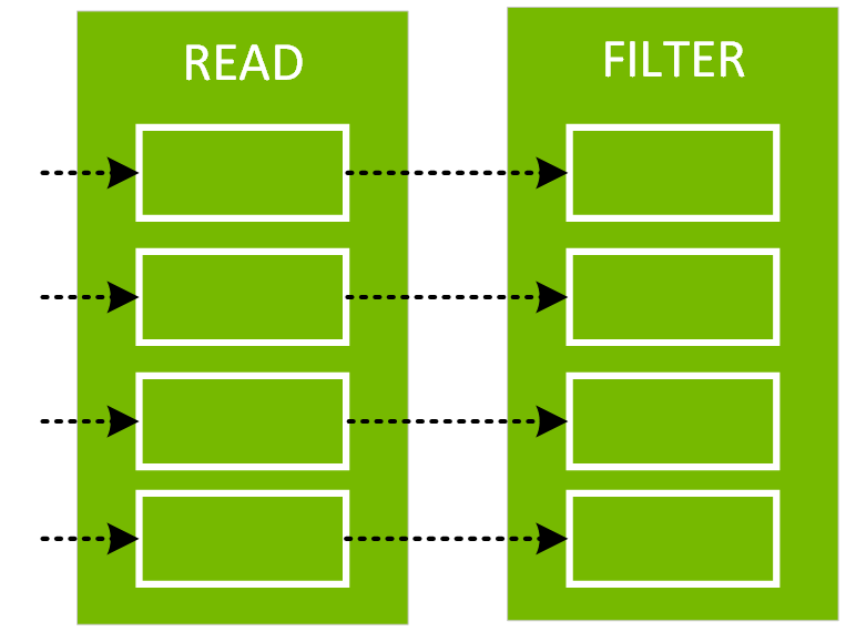
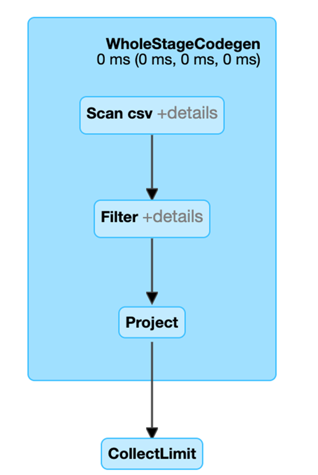
You can see the formatted physical plan for a DataFrame by calling the explain(“formatted”) method. In the physical plan below, the DAG for df2 consists of a Scan csv file, a Filter on day_of_week, and a Project (selecting columns) on hour, fare_amount, and day_of_week.
val df = spark.read.option("inferSchema", "false") .option("header", true).schema(schema).csv(file)
val df2 = df.select($"hour", $"fare_amount", $"day_of_week").filter($"day_of_week" === "6.0" )
df2.show(3)
result:
+----+-----------+-----------+
|hour|fare_amount|day_of_week|
+----+-----------+-----------+
|10.0| 11.5| 6.0|
|10.0| 5.5| 6.0|
|10.0| 13.0| 6.0|
+----+-----------+-----------+
df2.explain(“formatted”)
result:
== Physical Plan ==
* Project (3)
+- * Filter (2)
+- Scan csv (1)
(1) Scan csv
Location: [dbfs:/FileStore/tables/taxi_tsmall.csv]
Output [3]: [fare_amount#143, hour#144, day_of_week#148]
PushedFilters: [IsNotNull(day_of_week), EqualTo(day_of_week,6.0)]
(2) Filter [codegen id : 1]
Input [3]: [fare_amount#143, hour#144, day_of_week#148]
Condition : (isnotnull(day_of_week#148) AND (day_of_week#148 = 6.0))
(3) Project [codegen id : 1]
Output [3]: [hour#144, fare_amount#143, day_of_week#148]
Input [3]: [fare_amount#143, hour#144, day_of_week#148]
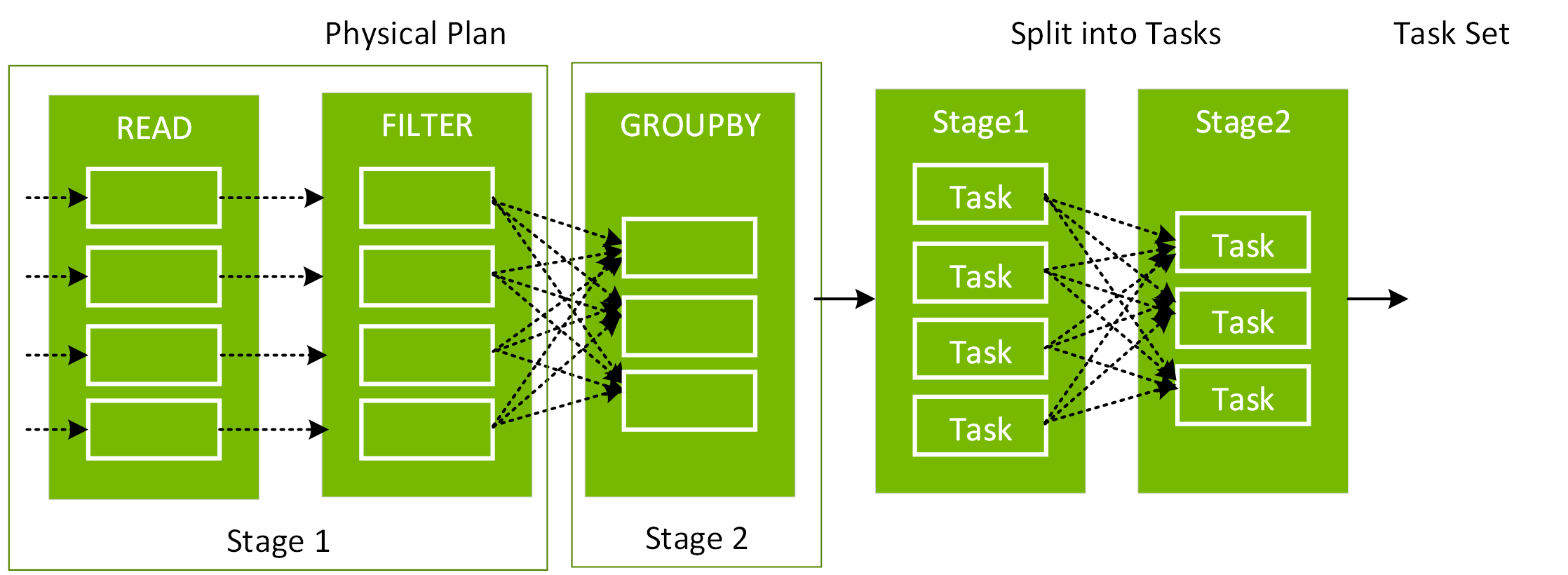
You can see more details about the plan produced by Catalyst on the web UI SQL tab. Clicking on the query description link displays the DAG and details for the query.
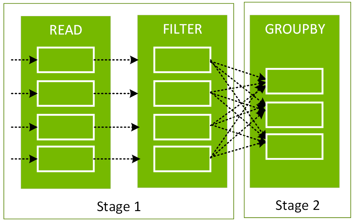
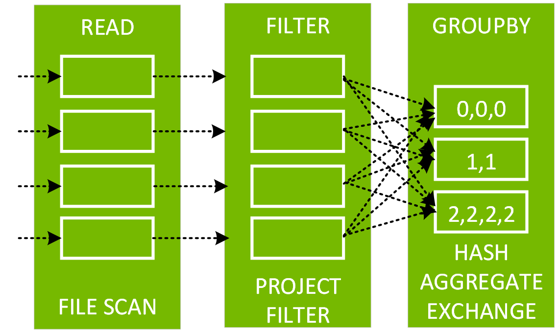
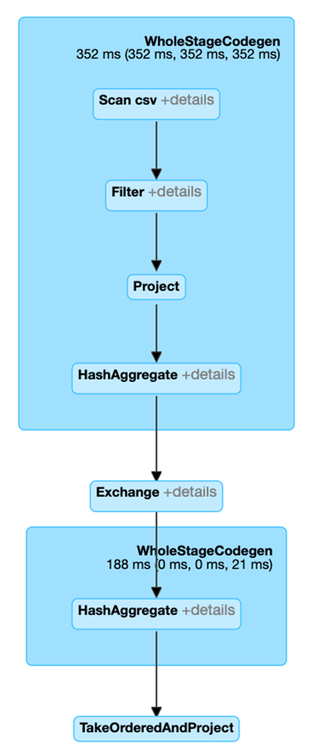
In the following code, after the explain, we see that the physical plan for df3 consists of a Scan, Filter, Project, HashAggregate, Exchange, and HashAggregate. The Exchange is the shuffle caused by the groupBy transformation. Spark performs a hash aggregation for each partition before shuffling the data in the Exchange. After the exchange, there is a hash aggregation of the previous sub-aggregations. Note that we would have an in-memory scan instead of a file scan in this DAG, if df2 were cached.
val df3 = df2.groupBy("hour").count
df3.orderBy(asc("hour"))show(5)
result:
+----+-----+
|hour|count|
+----+-----+
| 0.0| 12|
| 1.0| 47|
| 2.0| 658|
| 3.0| 742|
| 4.0| 812|
+----+-----+
df3.explain
result:
== Physical Plan ==
* HashAggregate (6)
+- Exchange (5)
+- * HashAggregate (4)
+- * Project (3)
+- * Filter (2)
+- Scan csv (1)
(1) Scan csv
Output [2]: [hour, day_of_week]
(2) Filter [codegen id : 1]
Input [2]: [hour, day_of_week]
Condition : (isnotnull(day_of_week) AND (day_of_week = 6.0))
(3) Project [codegen id : 1]
Output [1]: [hour]
Input [2]: [hour, day_of_week]
(4) HashAggregate [codegen id : 1]
Input [1]: [hour]
Functions [1]: [partial_count(1) AS count]
Aggregate Attributes [1]: [count]
Results [2]: [hour, count]
(5) Exchange
Input [2]: [hour, count]
Arguments: hashpartitioning(hour, 200), true, [id=]
(6) HashAggregate [codegen id : 2]
Input [2]: [hour, count]
Keys [1]: [hour]
Functions [1]: [finalmerge_count(merge count) AS count(1)]
Aggregate Attributes [1]: [count(1)]
Results [2]: [hour, count(1) AS count]
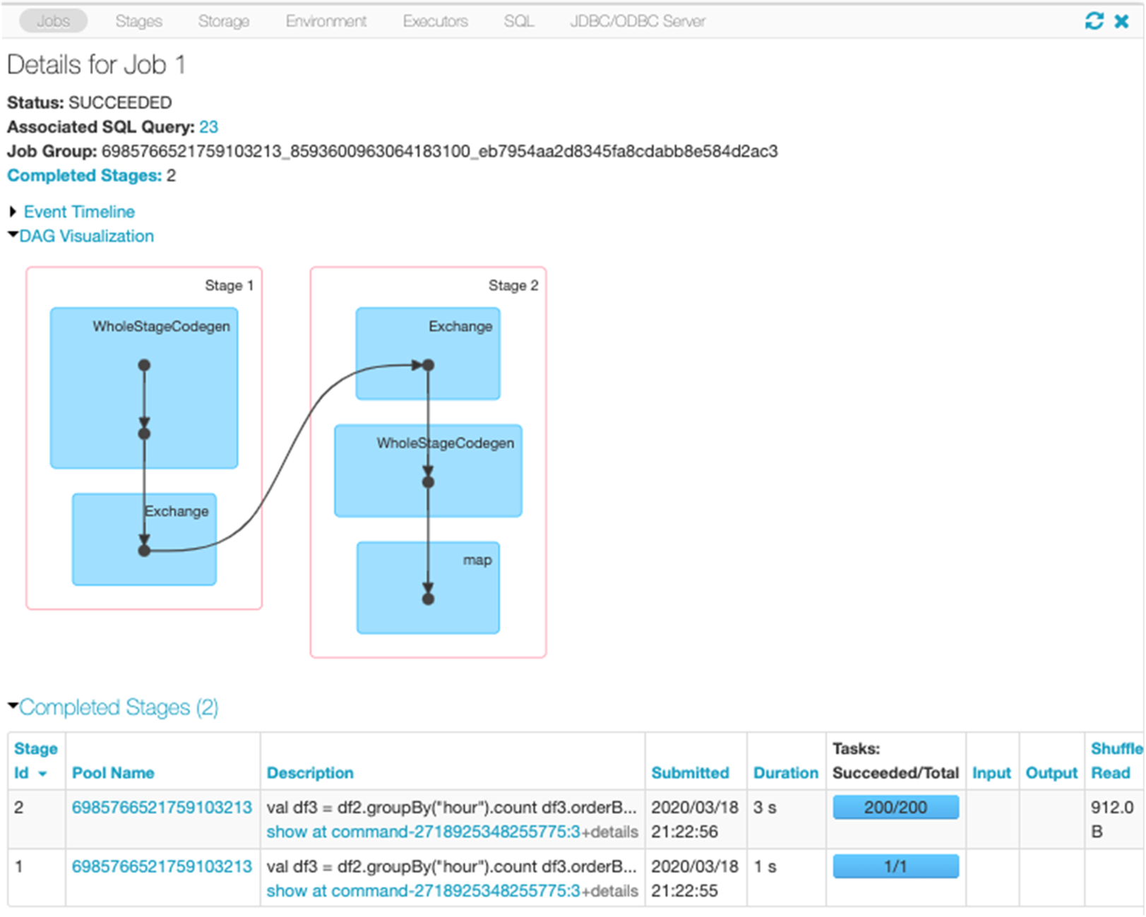
Clicking on the SQL tab link for this query display the DAG of the job.
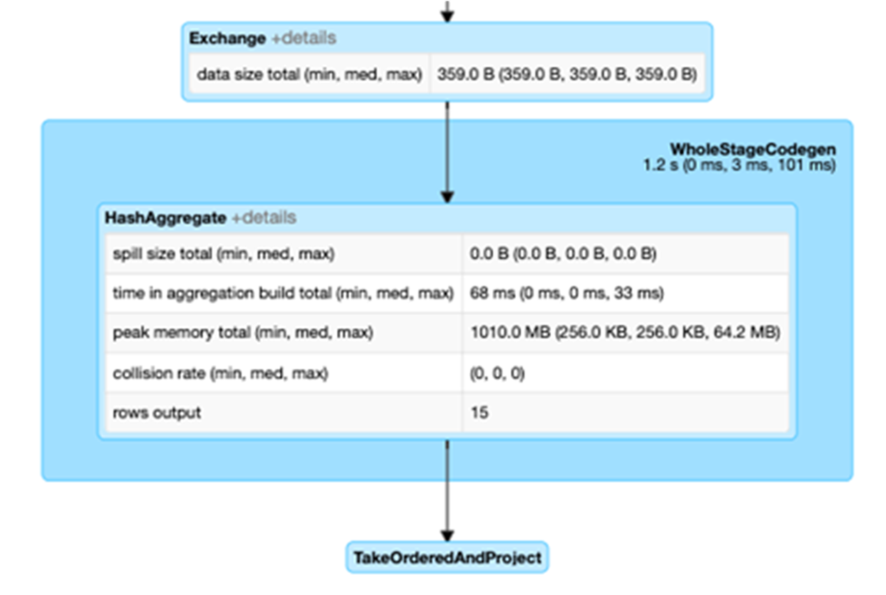
Selecting the Expand details checkbox shows detailed information for each stage. The first block WholeStageCodegen compiles multiple operators (scan csv, filter, project, and HashAggregate) together into a single Java function to improve performance. Metrics such as number of rows and spill size are shown in the following screen.
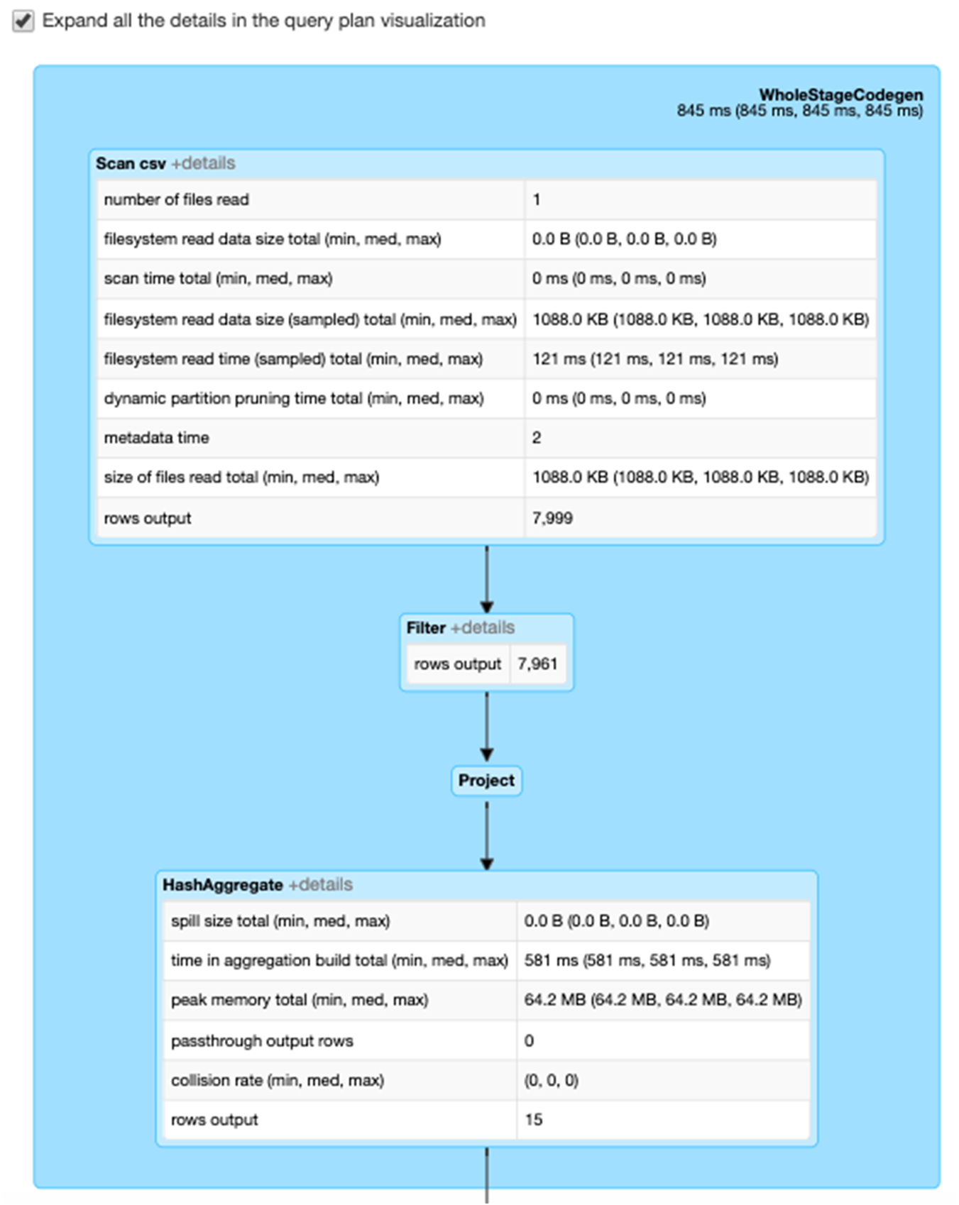
The second block entitled Exchange shows the metrics on the shuffle exchange, including the number of written shuffle records and the data size total.